Keyword [Mobilenet]
Howard A G, Zhu M, Chen B, et al. Mobilenets: Efficient convolutional neural networks for mobile vision applications[J]. arXiv preprint arXiv:1704.04861, 2017.
1. Overview
1.1. Motivation
- DNN become deeper and more complicated to achieve higher accuracy
- computational limited platform in reality
In this paper, it proposed an efficient model called MobileNet
- split standard Conv into depthwise Conv and pointwise Conv
- introduce two hyperparameter to trade off between latency and accuracy
- experiment on object detection, finegrain classification, face attributes and large scale geo-localization
1.2. Dataset
- Stanford Dogs
- YFCC100M (Yahoo Flickr Creative Commons 100 Million)
1.3. Related Work
most work
- compress pretrained networks
- train small networks directly
- depthwise separable Conv
- Flattened Networks
- Factorized Network
- Xception Network
- SqueezeNet
- Structured Transform Networks
- Deep Fried Convnets
- hasing
- pruning, vector quantization and Huffman coding
- distillation. using large model train small model instead of gt
low bit networks
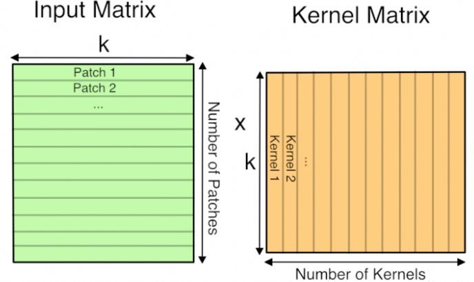
Convolution operations are Implemented by GEMM (general matrix multiply) which makes the kernel and input feature into two matrix and do matrix multiply.
- PlaNet. divide earth into a grid of geography cells, then do geolocation classification on images
2. Architecture
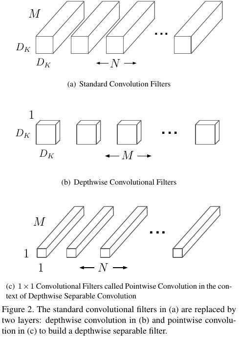
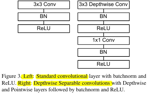
2.1. Depthwise Separable Conv
2.1.1. Standard Conv

- There exists the interaction between N and K.
- K. kernel size
- F. feature size
- M. input channel
- N. output channel
2.1.2. Depthwise Separable
- Depthwise Conv (KxKxM -> FxFxM). one kernel for one feature map.
- Pointwise Conv (1x1xMxN * FxFxM). the whole pointwise kernel for the whole output feature map of depthwise conv.

It breaks the interaction between the number of output channel and the size of the kernel.
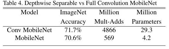
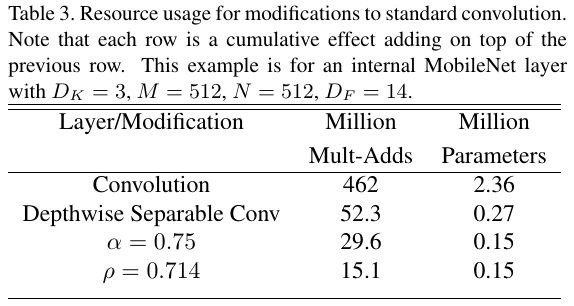
2.1.3. Comparison

for 3x3 kernel, 8~9 time less.
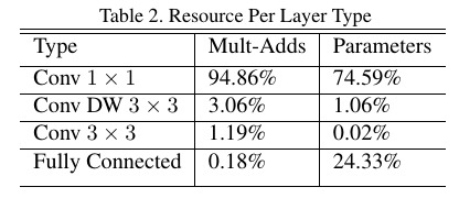
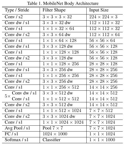
2.2. Structure
Mose computation time are in 1x1 Conv
Small model has less trouble with overfitting. It is important to put very little or no weight decay on depthwise filter.
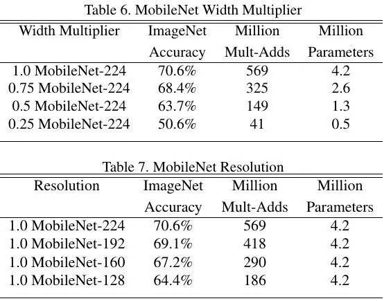
2.3. Hyperparameter
- Width Multiplier (α). Thinner Model (channel number)
- Resolution Multiplier (ρ). Reduced Representation (input size)

3. Experiments
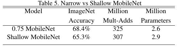
3.1. Thinner or Shallow
Thinner is better than Shallow.
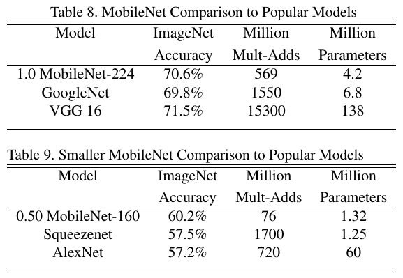
3.2. Comparison
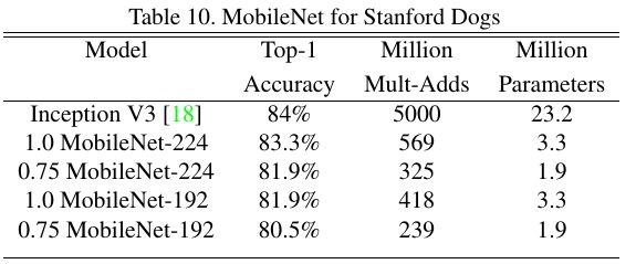
3.3. Stanford Dogs
3.4. Geolocalization
